From model to production

The Practice of Deep Learning

• Overestimating the constraints and underestimating the capabilities of deep learning may mean you do not attempt a solvable problem because you talk yourself out of it.
• The goal is not to find the “perfect” dataset or project, but just to get started and iterate from there.

Gathering Data

• Preparation:

!pip install -q fastbook fastai ipywidgets jupyterlab_widgets voila

from fastbook import *
from fastai.vision.widgets import *

import ipywidgets as widgets

• Download dataset from Bing using Azure Image API:

key = 'XXX' # Azure Search Images API Key

bear_types = 'grizzly', 'black', 'teddy'
path = Path('bears')

if not path.exists():
    path.mkdir()
    for o in bear_types:
        dest = (path/o)
        dest.mkdir(exist_ok=True)
        results = search_images_bing(key, f'{o} bear')
        download_images(dest, urls=results.attrgot('contentUrl'))

• Get the image files:

fns = get_image_files(path)
fns

• Find images in path that cannot be open and delete them

failed = verify_images(fns)
failed

failed.map(Path.unlink);

From Data to DataLoaders

• DataLoaders is a thin class that just stores whatever DataLoader objects you pass to it and makes them available as train and valid. It provides the data for your model.
• DataLoaders is the prepared data ready to be used for training:
  • Splitting the data into batches.
  • Applying transformations at the batch level.
  • Feeding batches to the model.

You create DataLoaders from a DataBlock or directly from your data.

• To turn our downloaded data into a DataLoaders object, we need to tell fastai at least four things:
  • What kinds of data we are working with.
  • How to get the list of items.
  • How to label these items.
  • How to create the validation set.
• The DataBlock is a high-level, flexible abstraction used to define how data should be processed and structured. It represents the blueprint for creating datasets and involves specifying:
  • What the data is: Types of inputs (e.g., images, texts) and labels.
  • How to get it: Where the data resides (e.g., folder, CSV, etc.).
  • How to transform it: Preprocessing (e.g., resizing, tokenization) and augmentations.
• Create data block:

bears = DataBlock(
    blocks=(ImageBlock, CategoryBlock),
    get_items=get_image_files,
    splitter=RandomSplitter(valid_pct=0.2, seed=42),
    get_y=parent_label,
    item_tfms=Resize(128)
)

• DataBlock:
  • blocks=(ImageBlock, CategoryBlock): A tuple specifying the types we want for the independent (images) and dependent (categories) variables. The independent (image) variable is often referred to as x, and the dependent (category) variable is often referred to as y.

  The independent variable is the thing we are using to make predictions from (images), and the dependent variable is our target (categories). In this case, our independent variable is a set of images, and our dependent variables are the categories (type of bear) for each image.

  • get_image_files: Takes a path, and returns a list of all of the images in that path (recursively, by default). Datasets usually include a validation set, either by organizing images into separate folders or providing a CSV file with filenames and dataset labels. fastai simplifies this by offering built-in classes or letting you create your own method.

  Often, datasets that you download will already have a validation set defined. Sometimes this is done by placing the images for the training and validation sets into different folders. Sometimes it is done by providing a CSV file in which each filename is listed along with which dataset it should be in. There are many ways that this can be done, and fastai provides a general approach that allows you to use one of its predefined classes for this or to write your own.

  • splitter=RandomSplitter(valid_pct=0.2, seed=42): We want to randomly split our training and validation sets but keep the same split each time we run the notebook. To do this, we set a fixed random seed. This ensures that the sequence of “random” numbers generated is the same every time, producing consistent splits.

  In this case, we want to split our training and validation sets randomly. However, we would like to have the same training/validation split each time we run this notebook, so we fix the random seed (computers don’t really know how to create random numbers at all, but simply create lists of numbers that look random; if you provide the same starting point for that list each time—called the seed—then you will get the exact same list each time)

  • get_y=parent_label: Gets the name of the folder a file is in. Because we put each of our bear images into folders based on the type of bear, this is going to give us the labels that we need.
  • item_tfms=Resize(128): We don’t feed the model one image at a time but several of them (what we call a mini-batch). To group them in a big array (usually called a tensor) that is going to go through our model, they all need to be of the same size. So, we need to add a transform that will resize these images to the same size. Item transforms are pieces of code that run on each individual item, whether it be an image, category, or so forth. fastai includes many predefined transforms; we use the Resize transform here and specify a size of 128 pixels.
• DataBlock object is like a template for creating a DataLoaders. We still need to tell fastai the actual source of our data—in this case, the path where the images can be found:

dls = bears.dataloaders(path)

• A DataLoader is a class that provides batches of a few items at a time to the GPU.
• A DataLoaders includes validation and training DataLoaders.
• When you loop through a DataLoader, fastai will give you 64 (by default) items at a time, all stacked up into a single tensor.
• Use show_batch to take a look at a few of the stacked up items:

dls.valid.show_batch(max_n=4, nrows=1)

• By default, Resize crops the images to fit a square shape of the size requested, using the full width or height. This can result in losing some important details. Alternatively, you can ask fastai to pad the images with zeros (black), or squish (stretch) them:

# Squish (strech)
bears = bears.new(item_tfms=Resize(128, ResizeMethod.Squish)) 
dls = bears.dataloaders(path)

dls.valid.show_batch(max_n=4, nrows=1)

# Padding
bears = bears.new(item_tfms=Resize(128, ResizeMethod.Pad, pad_mode='zeros')) 

dls = bears.dataloaders(path)
dls.valid.show_batch(max_n=4, nrows=1)

• All of these approaches have drawbacks:
  • Squishing (stretching) images distorts their shapes, leading to unrealistic representations and potentially causing the model to learn inaccuracies, which could lower accuracy.
  • Cropping removes important features, reducing the model's ability to perform accurate recognition.
  • Padding adds empty space, which wastes computational resources and lowers the effective resolution of the usable part of the image.
• The best approach is to randomly select a portion of the image and crop to that part. In each epoch (a complete pass through the dataset), we randomly select a different portion of each image, improving generalization and robustness.
• Training the neural network with examples of images in which the objects are in slightly different places and are slightly different sizes helps it to understand the basic concept of what an object is, and how it can be represented in an image.

bears = bears.new(
	item_tfms=RandomResizedCrop(128, min_scale=0.3)
)
dls = bears.dataloaders(path)

dls.train.show_batch(max_n=4, nrows=1, unique=True)

min_scale: Determines how much of the image to select at minimum each time. unique: to have the same image repeated with different versions of this RandomResizedCrop transform.

Data Augmentation

• Data augmentation: refers to creating random variations of our input data, such that they appear different but do not change the meaning of the data. Examples: rotation, flipping, perspective warping, brightness changes, and contrast changes.
• For natural photo images such as the ones we are using here, a standard set of augmentations that we have found work pretty well are provided with the aug_transforms function:

bears = bears.new(
    item_tfms=Resize(128), 
    batch_tfms=aug_transforms(mult=2)
)

dls = bears.dataloaders(path)
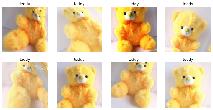
dls.train.show_batch(max_n=8, nrows=2, unique=True)

When you use the .new() method on a DataBlock, it creates a new DataBlock object that inherits the properties of the original DataBlock but allows you to modify specific parameters.

Training

bears = bears.new(
	item_tfms=RandomResizedCrop(224, min_scale=0.5),
	batch_tfms=aug_transforms()
) 
dls = bears.dataloaders(path)

learn = vision_learner(dls, resnet18, metrics=error_rate) 
learn.fine_tune(4)

Confusion Matrix

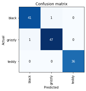
• The confusion matrix is a tool used in machine learning to evaluate the performance of a classification model. It shows the actual versus the predicted classifications made by the model.
• To visualize how our model is, we can create a confusion matrix:

interp = ClassificationInterpretation.from_learner(learn)
interp.plot_confusion_matrix()

• The rows represent all the black, grizzly, and teddy bears in our dataset, respectively.
• The diagonal of the matrix shows the images that were classified correctly, and the off-diagonal cells represent those that were classified incorrectly.

In the context of a confusion matrix, the "diagonal" refers to the cells that run from the top left corner to the bottom right corner of the matrix. These cells represent instances where the predicted class matches the actual class. Specifically, each cell on the diagonal indicates the number of correct predictions for each class.

• The diagonal of the matrix shows the images that were classified correctly, and the off-diagonal cells represent those that were classified incorrectly.
• This is one of the many ways that fastai allows you to view the results of your model. It is (of course!) calculated using the validation set.
• The goal is to have white everywhere except the diagonal, where we want dark blue.

Visualize the predictions

• We can sort our images by their loss to know where exactly our errors are occurring, to see whether they’re due to a dataset problem (e.g., images that aren’t bears at all, or are labeled incorrectly) or a model problem (perhaps it isn’t handling images taken with unusual lighting, or from a different angle, etc.).

The loss is a number that is higher if the model is incorrect (especially if it’s also confident of its incorrect answer), or if it’s correct but not confident of its correct answer.

• plot_top_losses: shows us the images with the highest loss in our dataset.

interp.plot_top_losses(5, nrows=1)

• This output shows that the image with the highest loss is one that has been predicted as “grizzly” with high confidence. However, it’s labeled (based on our Bing image search) as “black.”

Cleaning

• The intuitive approach to doing data cleaning is to do it before you train a model.
• We normally prefer to train a quick and simple model first, and then use it to help us with data cleaning.
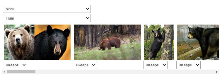
• fastai includes a handy GUI for data cleaning called ImageClassifierCleaner that allows you to choose a category and the training versus validation set and view the highest-loss images (in order), along with menus to allow images to be selected for removal or relabeling:

cleaner = ImageClassifierCleaner(learn) 
cleaner

ImageClassifierCleaner doesn’t do the deleting or changing of labels for you; it just returns the indices of items to change.

• To delete (unlink) all images selected for deletion, we would run this:

for idx in cleaner.delete(): cleaner.fns[idx].unlink()

• To move images for which we’ve selected a different category, we would run this:

for idx,cat in cleaner.change():
    shutil.move(str(cleaner.fns[idx]), path/cat)

Cleaning the data and getting it ready for your model are two of the biggest challenges for data scientists; they say it takes 90% of their time. If you delete images from your dataset after using ImageClassifierCleaner in fastai, you should re-train your model. The ImageClassifierCleaner tool is used to inspect and clean your dataset, often by removing incorrectly labeled or noisy images.

Using the Model for Inference

• A model consists of two parts: the architecture and the trained parameters. The easiest way to save a model is to save both of these, because that way, when you load the model, you can be sure that you have the matching architecture and parameters. To save both parts, use the export method.
• fastai automatically uses your validation set DataLoader for inference by default.

When we use a model for getting predictions, instead of training, we call it inference. "inference" refers to the process of using a trained model to make predictions on new, unseen data.

• Export the model:

learn.export()

• To create our inference learner from the exported file, we use load_learner:

learn_inf = load_learner(path/'export.pkl')

learn_inf.predict('images/grizzly.jpg')

# ('grizzly', tensor(1), tensor([9.0767e-06, 9.9999e-01, 1.5748e-07]))

• This has returned three things: the predicted category in the same format you originally provided (in this case, that’s a string), the index of the predicted category, and the probabilities of each category. The last two are based on the order of categories in the vocab of the DataLoaders; that is, the stored list of all possible categories:

learn_inf.dls.vocab

# (#3) ['black','grizzly','teddy']

Deploying Your App

• You need a GPU to train nearly any useful deep learning model. So, do you need a GPU to use that model in production? No! You almost certainly do not need a GPU to serve your model in production.

Some very large models, such as LLMs, or those requiring real-time inference with very low latency might still benefit from GPU acceleration in production.

• We recommend wherever possible that you deploy the model itself to a server, and have your mobile or edge application connect to it as a web service.

Horizontal scaling involves adding more machines to a system (scaling out), while vertical scaling involves adding more power (CPU, RAM) to an existing machine (scaling up). Horizontal scaling improves capacity and redundancy, while vertical scaling enhances the performance of a single node.

How to Avoid Disaster

• One of the biggest issues to consider is that understanding and testing the behavior of a deep learning model is much more difficult than with most other code you write.
• With normal software development, you can analyze the exact steps that the software is taking, and carefully study which of these steps match the desired behavior that you are trying to create. But with a neural network, the behavior emerges from the model’s attempt to match the training data, rather than being exactly defined.
• There may be data that our model sees in production that is very different from what it saw during training. There isn’t a complete technical solution to this problem; instead, we have to be careful about our approach to rolling out the technology.
• This can result in disaster! For instance, let’s say we really were rolling out a bear detection system that will be attached to video cameras around campsites in national parks and will warn campers of incoming bears. If we used a model trained with the dataset we downloaded, there would be all kinds of problems in practice, such as these:
  • Working with video data instead of images
  • Handling nighttime images, which may not appear in this dataset
  • Dealing with low-resolution camera images
  • Ensuring results are returned fast enough to be useful in practice
  • Recognizing bears in positions that are rarely seen in photos that people post online (for example from behind, partially covered by bushes, or a long way away from the camera)
• This is just one example of the more general problem of out-of-domain data. That is to say, there may be data that our model sees in production that is very different from what it saw during training. There isn’t a complete technical solution to this problem; instead, we have to be careful about our approach to rolling out the technology.

Out-of-domain data refers to data that is outside the scope or context of the data that a model was trained on or is typically designed to handle. In machine learning and natural language processing, this can lead to poor performance because the model has not been exposed to this type of data during training, and thus may not understand or predict it accurately.

• There are other reasons we need to be careful too. One very common problem is domain shift, whereby the type of data that our model sees changes over time. For instance, an insurance company may use a deep learning model as part of its pricing and risk algorithm, but over time the types of customers the company attracts and the types of risks it represents may change so much that the original training data is no longer relevant.
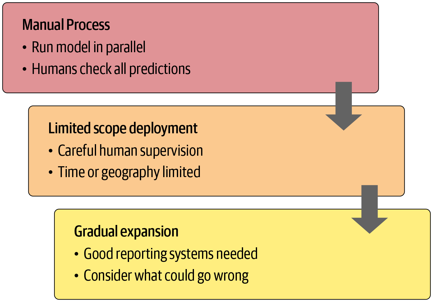
• The good news, however, is that there are ways to mitigate these risks using a carefully thought-out process:
• The humans involved in the manual process should look at the deep learning outputs and check whether they make sense.

Unforeseen Consequences and Feedback Loops

• One of the biggest challenges in rolling out a model is that your model may change the behavior of the system it is a part of.
• For instance, Predictive policing algorithms don’t predict crime itself but rather reinforce patterns of police deployment. They direct more police to areas with historically high police activity, resulting in more recorded crimes and perpetuating the cycle. This shifts the focus from forecasting crime to reinforcing existing biases in police presence.

Predictive policing uses data analysis and algorithms to forecast where crimes are likely to occur or who might commit them. It analyzes historical crime data to guide police deployment, aiming to prevent crime proactively. However, it often raises concerns about reinforcing biases and perpetuating over-policing in certain communities.

• Feedback loops can result in negative implications of that bias getting worse and worse. For instance, there are concerns that this is already happening in the US, where there is significant bias in arrest rates on racial grounds.
• Bärí Williams wrote in the New York Times: “The same technology that’s the source of so much excitement in my career is being used in law enforcement in ways that could mean that in the coming years, my son, who is 7 now, is more likely to be profiled or arrested—or worse—for no reason other than his race and where we live.”
• A feedback loop is a process where the output of a system influences its own input, creating a cycle of effects. This can either amplify (positive feedback) or stabilize (negative feedback) the system's behavior.
• A helpful exercise prior to rolling out a significant machine learning system is to consider this question: “What would happen if it went really, really well?” In other words, what if the predictive power was extremely high, and its ability to influence behavior was extremely significant? In that case, who would be most impacted? What would the most extreme results potentially look like? How would you know what was really going on?

Make sure that reliable and resilient communication channels exist so that the right people will be aware of issues and will have the power to fix them.