All you need to know about NumPy

• NumPy is a tool that helps computers quickly and easily handle large amounts of numbers. This is really useful for things like working with images and videos, which are made up of many numbers (pixels). By using NumPy, we can perform complex calculations and processes more efficiently, making our programs run faster.
• While Python lists can include many different data types, all of the elements in a NumPy array must be the same data type. This makes NumPy very efficient: there's no need for NumPy to check the data type of each element in an array since they must all be the same. Having only a single data type also means that a NumPy array takes up less space in memory than the same information would if stored as a Python list.

import numpy as np

# Create a numpy array from Python list
python_list = [3, 2, 5, 8, 4, 9, 6, 1]
array = np.array(python_list)

# Array with zeros
np.zeros((3, 3))

# Random
np.random.random((3, 3))

# Create evenly-spaced array
np.arange(-3, 4) # [-3, -2, -1, 0, 1, 2, 3]

• Programmers and the NumPy documentation sometimes refer to arrays as vectors, matrices, or tensors. These are mathematical terms rather than NumPy terms; they all describe types of arrays. The difference between them is the number of dimensions an array has.
• A vector refers to an array with one dimension.
• In mathematics, a two-dimensional array is called a matrix. And an array with three or more dimensions is called a tensor.

# 1D array (vector)
[1, 2, 3, 4, 5]

# 2D array (matrix)
[
	[1, 2, 3], 
	[4, 5, 6]
]

# 3D array (tensor)
[
	[
		[1, 2, 3], 
		[4, 5, 6]
	], 
	[
		[7, 8, 9], 
		[10, 11, 12]
	]
]

In NumPy, 1D arrays are a special case where the concept of rows and columns doesn't strictly apply. A 1D array has a shape of (n,), where n is the number of elements. There's no second dimension specified.

Homogeneous

• Numpy arrays are considered homogeneous because, in general, each element in a Numpy array is of the same type. This homogeneity is what gives Numpy arrays their efficiency, especially in numerical computations. When Numpy arrays are homogeneous, operations can be optimized because the underlying memory layout is predictable and contiguous.
• When you create a Numpy array with dtype=object, it technically breaks the usual homogeneity of the array. The elements are no longer stored as a fixed data type but as references to Python objects, which can be of different types. This is why operations on object arrays are slower and less efficient compared to regular Numpy arrays:

np_objects = np.array([
    ['1986', 'Ahmad', 181.0, 78]
], dtype=object)

print(np_objects)

Array Attributes

• NumPy arrays have several attributes that provide information about the array. Here are some commonly used attributes of NumPy arrays:
  • shape: This attribute returns a tuple representing the shape of the array, i.e., the number of elements along each dimension.
  • ndim: This attribute returns the number of dimensions of the array.
  • size: This attribute returns the total number of elements in the array.
  • dtype: This attribute returns the data type of the elements in the array.
  • itemsize: This attribute returns the size in bytes of each element in the array.
  • data: This attribute returns a buffer object pointing to the start of the array's data.

Array Methods

• flatten: it takes all array elements and puts them in just one dimension inside a 1D array.

arr = np.array([[1, 2], [3, 4]]
arr.flatten() # [1, 2, 3, 4]

• reshape: allows us to redefine the shape of an array without changing the elements that make up the array. The shape tuple must be compatible with the number of elements in an array.

arr = np.array([[1, 2, 3], [4, 5, 6]])
arr.reshape((3,2)) # [[1 2] [3 4] [5 6]]

• stack: stack arrays along a new axis. This means that it takes a sequence of arrays and stacks them along a new axis, which increases the dimensionality of the resulting array:

import numpy as np

# Create two arrays
arr1 = np.array([1, 2, 3])
arr2 = np.array([4, 5, 6])

# Stack the arrays along a new axis
stacked_array = np.stack((arr1, arr2))

print(stacked_array)
#[[1 2 3]
# [4 5 6]]

• astype: type conversion:

boolean_array = np.array(
    [[True, False], [False, False]], dtype=np.bool_)
boolean_array.astype(np.int32)

What is an Axis in NumPy?

• An axis is like a direction along which we can perform operations on arrays. Imagine an array as a grid or table of numbers.
• The axes are the directions along which the data is organized.
  • Axis 0 is the direction down the rows (like moving vertically).
  • Axis 1 is the direction across the columns (like moving horizontally).
• If you think of a 2D array (a matrix), then:
  • Axis 0 goes down the rows.
  • Axis 1 goes across the columns.
• The number of axes depends on the number of dimensions in the array.
• 1D Array (1 Axis):

arr_1d = np.array([1, 2, 3])

# Axis 0: The only axis in a 1D array
sum_axis_0 = np.sum(arr_1d, axis=0)  # Output: 6

• 2D Array (2 Axis):

# Creating a 2D array (2x3)
arr_2d = np.array([[1, 2, 3], [4, 5, 6]])

# Axis 0: Down the rows (sum along columns)
sum_axis_0 = np.sum(arr_2d, axis=0)  # Output: [5, 7, 9]

# Axis 1: Across the columns (sum along rows)
sum_axis_1 = np.sum(arr_2d, axis=1)  # Output: [6, 15]

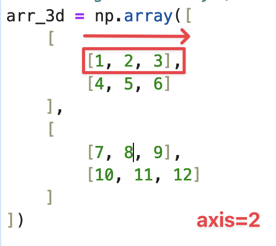
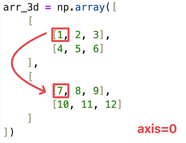
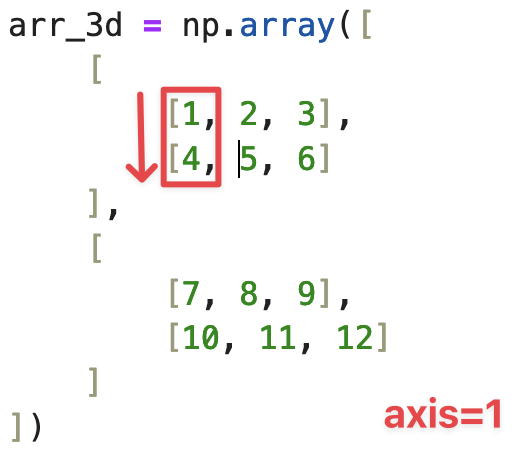
• 3D Array (3 Axes):

# Creating a 3D array (2x2x3)
arr_3d = np.array([[[1, 2, 3], [4, 5, 6]], 
                   [[7, 8, 9], [10, 11, 12]]])

# Axis 0: Along the depth (sum across 2D arrays)
sum_axis_0 = np.sum(arr_3d, axis=0)  # Output: [[ 8, 10, 12], [14, 16, 18]]

# Axis 1: Down the rows within each 2D array
sum_axis_1 = np.sum(arr_3d, axis=1)  # Output: [[ 5,  7,  9], [17, 19, 21]]

# Axis 2: Across the columns within each 2D array
sum_axis_2 = np.sum(arr_3d, axis=2)  # Output: [ 6, 15], [24, 33]]

The number of axes corresponds directly to the number of dimensions (or "rank") of that array. 1D Array: 1 axis (Axis 0). 2D Array: 2 axes (Axis 0, Axis 1). 3D Array: 3 axes (Axis 0, Axis 1, Axis 2). Etc...

Indexing and slicing arrays

• Accessing elements:

# Index
arr[0]

# Index 2D array (row, column)
arr[2, 4]

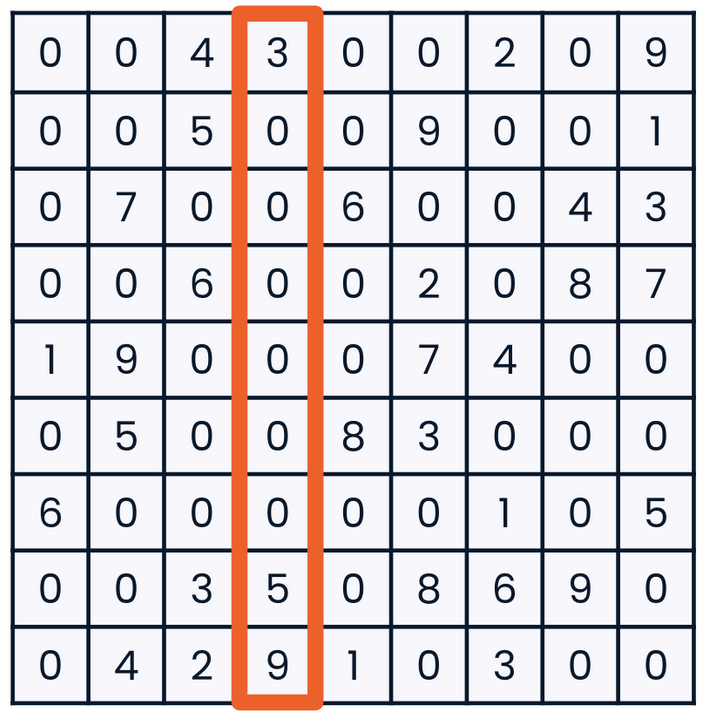
• Index a column: indicate a column index by providing a colon in place of any row index. The colon by itself tells NumPy that we are looking for all row information:

arr[:, 3]

• Slicing: extracts a subset of data based on given indices from one array and creates a new array with the sliced data:

array = np.array([2, 4, 6, 8, 10])
array[2:4] # Output: [6, 8]

The element at the start index is included in the result, but the one at the stop index is not: here, the number 10 at index four is excluded from the result.

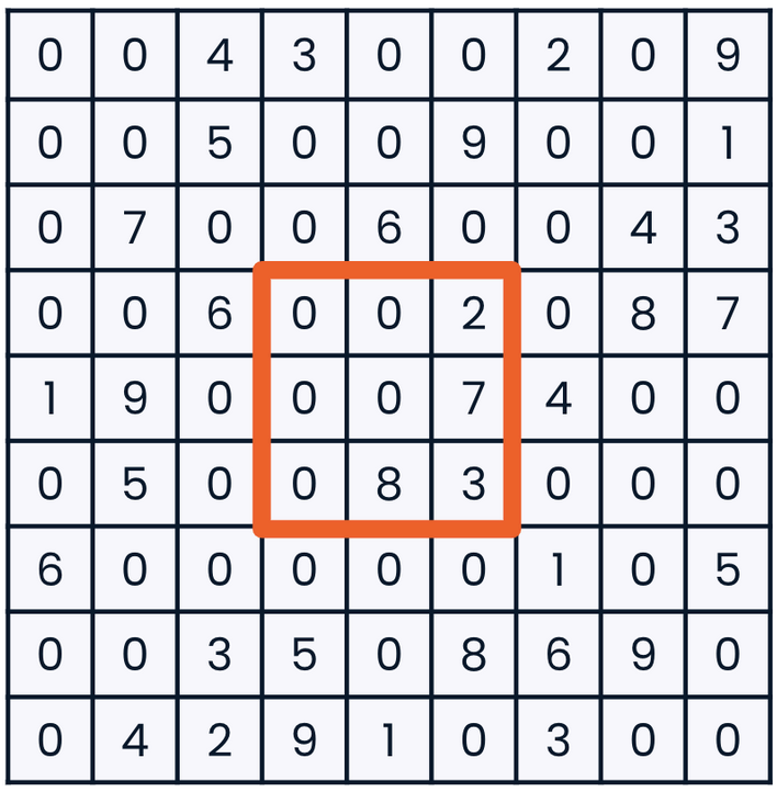
• Slicing 2D array: To slice in 2D, we'll need to give NumPy information on how both the rows and columns should be sliced:

arr[3:6, 3:6]

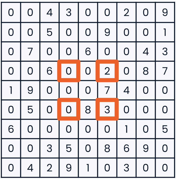
• Slicing with steps: we can give NumPy a third number: step value.

arr[3:6:2, 3:6:2]

• Sorting an array: By default, numpy.sort sorts each individual array along the specified axis, and it defaults to sorting along the last axis (i.e., axis=-1):

s = np.array([[2,6,9,1], [8,7,2,5]])
np.sort(s)
# array([[1, 2, 6, 9],
#	   [2, 5, 7, 8]])

• Axis Order: In a 2D array, the direction along rows is axis zero. The direction along columns is axis one. An easy way to remember that axis one refers to columns is that a column looks like the number one!
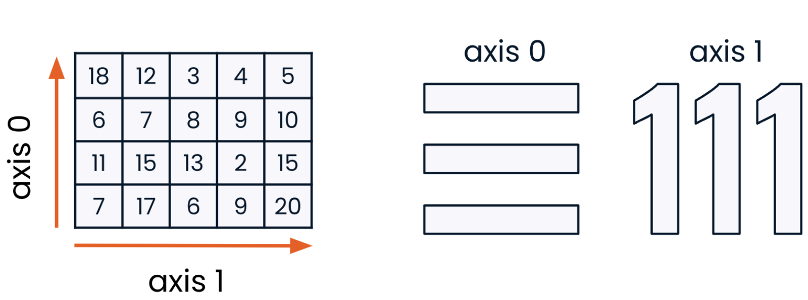
• Sort the array by row, so that the highest numbers in each column are at the bottom of the array:

np.sort(arr, axis=0)

Filtering

• Mask: A mask is a boolean array—an array of True or False values—that corresponds in shape to the array you want to filter. Each True value in the mask indicates that the corresponding element in the original array should be included in the filtered result, while False means it should be excluded, let’s create a mask that selects even numbers:

arr = np.array([1, 2, 3, 4, 5, 6, 7, 8, 9])

# Create a mask that selects even numbers
mask = arr % 2 == 0

# fancy indexing, which uses a Boolean mask to select 
# and return elements from an array that satisfy certain conditions
arr(mask)

• np.where: The np.where function in NumPy is a versatile tool that allows you to select elements from an array based on a condition:

arr = np.array([10, 15, 20, 25, 30])

# Find the indices of elements that are greater than 20
indices = np.where(arr > 20)

print(indices) # (array([3, 4]),)

Concatenation

arr1 = np.array([[1, 2], [3, 4], [5, 6]])
arr2 = np.array([[7, 8], [9, 10], [11, 12]])

np.concatenate((arr1, arr2), axis=1)

# array([[ 1,  2,  7,  8],
#	   [ 3,  4,  9, 10],
#	   [ 5,  6, 11, 12]])

The arrays to be concatenated must have compatible shapes. Specifically, they must have the same shape along all axes except the one being concatenated along.

• We can concatenate a three by three array with a three by two array column-wise, because the axis we are concatenating along, the second axis, is the only axis which does not have the same length:

arr1 = np.array([[1, 2, 3], [3, 4, 5], [5, 6, 7]])
arr2 = np.array([[7, 8], [9, 10], [11, 12]])

# This works because we concantenae on the axis 1 otherwise it'll fail
np.concatenate((arr1, arr2), axis=1)

# array([[ 1,  2,  3,  7,  8],
#       [ 3,  4,  5,  9, 10],
#       [ 5,  6,  7, 11, 12]])

• The two arrays must also have the same number of dimensions.

• It is not possible to add new dimensions with np.concatenate, since the function only adds data along an existing axis.
• Reshape: When concatenating arrays in NumPy, the dimensions and shapes of the arrays need to be compatible along the specified axis. If they are not compatible, you may need to reshape the arrays before concatenation.

# Original arrays with different shapes
arr1 = np.array([[1, 2], [3, 4]])  # Shape: (2, 2)
arr2 = np.array([5, 6])            # Shape: (2,)

# Reshape arr2 to have the same number of rows (axis 0) and match the columns
arr2_reshaped = arr2.reshape(2, 1)  # Shape: (2, 1)

Logical Operators

• np.logical_and: This function returns True where both inputs are True.

a = np.array([True, False, True])
b = np.array([True, True, False])

result = np.logical_and(a, b)
# Output: array([ True, False, False])

• np.logical_or: This function returns True where at least one of the inputs is True.

result = np.logical_or(a, b)

• np.logical_not: This function returns the logical negation of the input array (i.e., it flips True to False and vice versa).

result = np.logical_not(a)

• np.logical_xor: This function returns True where the inputs differ (i.e., one is True and the other is False).

result = np.logical_xor(a, b)

Deleting

• np.delete function takes three arguments: the array to delete from, a slice, index, or array of indices to be deleted, and the axis to be deleted along. For example, to delete the second row from a 2D array, the index to delete will be one, and the deletion will occur along the first axis, represented with a zero:

# Delete number 5
arr = np.array([[1, 2, 3], [3, 4, 5], [5, 6, 7]])
arr_without_5 = np.delete(arr, np.where(arr == 5))
print(arr_without_5)

• To delete the second column instead, update the axis keyword argument to one. Now, our class size column is gone:

arr1 = np.array([[1, 2, 3], [4, 5, 6], [7, 8, 9]])

np.delete(arr1, 1, axis=1)

• If no axis is specified, NumPy deletes the indicated index or indices along a flattened version of the array:

arr1 = np.array([[1, 2, 3], [4, 5, 6], [7, 8, 9]])

np.delete(arr1, 1)

# array([1, 3, 4, 5, 6, 7, 8, 9])

Summarizing data

• np.sum(): Calculates the sum of array elements along a specified axis. By default the dimensions will be flattened to a 1D array:

# without axis (sum total)
array = np.array([[1, 2, 3],
                  [4, 5, 6],
                  [7, 8, 9]])

np.sum(array) # total: 45

np.sum(array, axis=0) # sum columns: array([12, 15, 18])

np.sum(array, axis=1) # sum rows: array([ 6, 15, 24])

np.sum(array, axis=0, keepdims=True) # array([[12, 15, 18]])

• np.mean(): Computes the arithmetic mean (average) of array elements along a specified axis.
• np.median(): Finds the median (middle value) of the array elements.
• np.std(): Computes the standard deviation, which measures the spread of data points.
• np.var(): Calculates the variance, which is the average of the squared deviations from the mean.
• np.min(): Finds the minimum value in the array.
• np.max(): Finds the maximum value in the array.
• np.prod(): Computes the product of array elements.
• np.cumsum(): Computes the cumulative sum of array elements along a given axis.
• np.cumprod(): Computes the cumulative product of array elements.
• np.percentile(): Computes the q-th percentile of the data along the specified axis.
• np.quantile(): Computes the quantile of the data along the specified axis.
• np.argmin(): Returns the indices of the minimum values along an axis.
• np.argmax(): Returns the indices of the maximum values along an axis.
• np.any(): Tests whether any array element along a given axis evaluates to True.
• np.all(): Tests whether all array elements along a given axis evaluate to True.
• np.unique(): Finds the unique elements in an array.

Vectorized operations

• Vectorized operations in NumPy refer to performing operations on entire arrays (or large blocks of data) at once, rather than using explicit loops. This approach leverages optimized, low-level implementations in C and takes advantage of hardware acceleration, resulting in significant performance improvements compared to iterative approaches in Python.
• Element-wise Operations: Suppose you have two arrays, and you want to perform element-wise addition:

# Create two arrays
a = np.array([1, 2, 3, 4])
b = np.array([5, 6, 7, 8])

# Element-wise addition
c = a + b # [ 6  8 10 12]

• Broadcasting: Broadcasting allows you to perform operations between arrays of different shapes. For instance, adding a scalar to an array:

# Create an array
a = np.array([1, 2, 3, 4])

# Add a scalar to the array
b = a + 10 # [11 12 13 14]

• Applying Functions Element-wise: Using universal functions to apply mathematical functions element-wise.

# Create an array
a = np.array([0, np.pi / 2, np.pi, 3 * np.pi / 2])

# Apply the sine function
b = np.sin(a)

• Operations on 2D Arrays: Performing operations on multi-dimensional arrays.

# Create a 2D array
matrix = np.array([[1, 2, 3],
                   [4, 5, 6]])

# Element-wise multiplication by 2
result = matrix * 2

# [[ 2  4  6]
# [ 8 10 12]]

While vectorized operations work extremely well with math and numbers, they are leveraged throughout NumPy; we used them to create Boolean masks and filter arrays.

• np.vectorize: is a function in NumPy that allows you to apply a scalar function to each element of an array in a vectorized manner. Essentially, it "vectorizes" a function, enabling it to operate element-wise on arrays as if it were naturally compatible with NumPy's broadcasting and array operations:

numpy.vectorize(pyfunc, otypes=None, doc=None, excluded=None, cache=False)

Example:

# Define a custom function
def square(x):
    return x ** 2

# Vectorize the function
vectorized_square = np.vectorize(square)

# Create an array
arr = np.array([1, 2, 3, 4, 5])

# Apply the vectorized function
result = vectorized_square(arr)

print(result)

Dimension Compatibility (Broadcasting) in NumPy

• Concept: Broadcasting allows arrays of different shapes to interact in arithmetic operations by extending smaller arrays to match larger ones.
• Rules:
  1. Align Dimensions: Pad smaller arrays with ones on the left if they have fewer dimensions.
  2. Dimension Compatibility: Dimensions are compatible if:
     1. They are the same, or.
     2. One of them is 1.
  3. Broadcasting: Extend arrays with size 1 to match the shape of the other array.
• Basic Broadcasting:

array1 = np.array([1, 2, 3])
array2 = np.array([[4], [5], [6]])
result = array1 + array2

# Output: [[5 6 7] [6 7 8] [7 8 9]]

• Different Shapes:

array1 = np.array([[1, 2, 3], [4, 5, 6]])
array2 = np.array([10, 20, 30])
result = array1 + array2
# Output: [[11 22 33] [14 25 36]]

• Higher-Dimensional:

array1 = np.array([1, 2, 3])
array2 = np.array([[4], [5], [6]])
array3 = np.array([10])
result = array1 + array2 + array3
# Output: [[15 16 17] [16 17 18] [17 18 19]]

Saving and loading arrays

import numpy as np
import matplotlib.pyplot as plt

# Create a 3x3 image with RGB values
rgb = np.array([
    [[255, 0, 0], [255, 0, 0], [255, 0, 0]],  # Red row
    [[0, 255, 0], [0, 255, 0], [0, 255, 0]],  # Green row
    [[0, 0, 255], [0, 0, 255], [0, 0, 255]]   # Blue row
])

# Display the image
plt.imshow(rgb)
plt.show()

• Save as npy:

with open("array.npy", "wb") as f:
    np.save('array.npy', rgb)

• Load npy:

with open("array.npy", "rb") as f:
    rgb_array = np.load(f)

• Access one RGB layer:

red = rgb[:, :, 0]
blue = rgb[:, :, 1]
green = rgb[:, :, 2]

Array acrobatics

• In machine learning, data augmentation is the process of adding additional data by performing small manipulations on data that is already available. For example, let's say we've got a dataset of a thousand images we are using to train a model classifying whether the items are recyclable or not. We could augment this data by flipping each image and use both the flipped and original images to train the model. This helps the model learn that image orientation isn't relevant to its classification as recyclable or not.
• np.flip: inverts the image along a specified axis.
• transpose: involves rearranging the axes of the image array. For a 2D image, transposing would switch the rows and columns, effectively rotating the image by 90 degrees. In the context of an image, transpose can also refer to a series of predefined operations such as rotating by specific angles (90°, 180°, 270°).

Stacking and splitting

• Recall that we can slice 3D RGB data to get red, green, and blue 2D arrays. Values in the red correspond to the red values from each pixel in the original array of all red, green, and blue values.

red = rgb[:, :, 0]
blue = rgb[:, :, 1]
green = rgb[:, :, 2]

• Splitting arrays: We can also unpack arrays using np-dot-split, a function which accepts three arguments: the array to split, the number of equally-sized arrays desired after the split, and the axis to split along.

r, b, g = np.split(rgb, 3, axis=2)

Random Number

• In NumPy, random numbers can be generated using the numpy.random module, which provides a wide variety of functions to generate random numbers and perform random sampling:

# Random Float Between 0 and 1

import numpy as np
random_number = np.random.rand()
print(random_number)

# Random Array of Floats Between 0 and 1:
random_array = np.random.rand(3, 2)  # 3x2 array of random floats
print(random_array)

# Random Integers:
random_integers = np.random.randint(1, 10, size=(3, 2))  # 3x2 array of random integers between 1 and 9
print(random_integers)

# Random Normal Distribution
random_normal = np.random.randn(5)  # 1D array of 5 random numbers from a normal distribution
print(random_normal)

# Random Choice from an Array
choices = np.random.choice([1, 2, 3, 4, 5], size=3)  # Randomly pick 3 elements from the list
print(choices)

• A seed in random number generation is a starting point for the sequence of random numbers. When you set a seed, you ensure that the sequence of random numbers generated is reproducible. This is useful for debugging, experiments, and when you want to ensure consistency in your results:

np.random.seed(42)  # Set the seed to 42
random_number = np.random.rand() # always same number
print(random_number)

• Once the seed is set, the sequence of random numbers generated will be the same every time you run the code. For example, if you run the above code snippet with the seed 42, you will always get the same random number.